Combining Senses and Predicting Them

Why can you not tickle yourself, when a stranger’s finger on the same spot makes you squirm? Two kinds of weighting answer it. A nervous system has to decide how much to trust each sense, and it has to decide how much of the input at its receptors is only the consequence of its own movement. This lesson starts where sensory coding stops: the spikes are already a code, and the question is what is done with several streams of them.

Two cues, one estimate

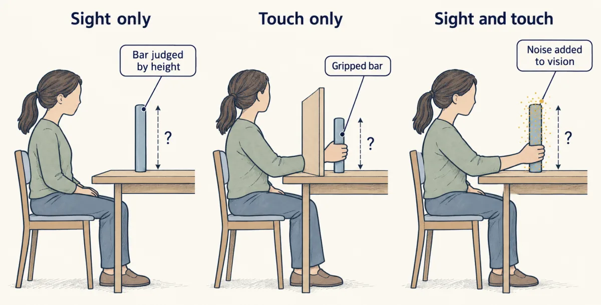
Suppose you judge the height of a bar by looking at it and by gripping it. Each sense gives a noisy estimate. If the noise in each is independent and Gaussian, the estimates are unbiased and you have no prior preference for any height, the combination with the least variance is a weighted average. Each weight is the cue’s precision (one over its variance) divided by the sum of the precisions:

w_V = (1/σV²) / (1/σV² + 1/σH²), w_H = 1 − w_V combined estimate = w_V × estimate_V + w_H × estimate_H combined variance = σV² σH² / (σV² + σH²)

Ernst and Banks (Nature, 2002) tested this with four human observers who judged bar height by sight and by touch. They made vision less reliable by adding noise to the visual stimulus and compared the combined judgements with predictions built from each observer’s single-sense performance. A maximum-likelihood model closely resembled the judgements. Read the scope: one task, four people, a behavioural fit. Agreement supports the model as a description of what observers do. It does not locate the weighting in the brain or show that every pair of cues is combined this way.

Alais and Burr (Current Biology, 2004) asked the same question for sound and sight in human localization. Vision usually dominates where a sound seems to come from, but when they blurred the visual stimulus severely, sound captured the perceived location of the visual one. So “vision wins” is a statement about typical reliability, not a law.

Worked problem (illustrative numbers). Take independent, unbiased Gaussian estimates of one bar height and a uniform prior. Vision has SD 2 mm and touch SD 4 mm. On one trial vision says 50 mm and touch says 54 mm.

1. Variances: 4 mm² and 16 mm². Precisions: 1/4 and 1/16 per mm².
2. Weights: w_V = (1/4)/(1/4 + 1/16) = 0.8 and w_H = 0.2.
3. Combined estimate: 0.8 × 50 + 0.2 × 54 = 50.8 mm.
4. Combined variance: (4 × 16)/(4 + 16) = 3.2 mm², so SD = 1.789 mm. Check: 0.8² × 4 + 0.2² × 16 = 2.56 + 0.64 = 3.2 mm².

The combined SD is lower than either cue alone. Now blur the picture until vision has SD 8 mm (variance 64 mm²). The weights become w_V = (1/64)/(1/64 + 1/16) = 0.2 and w_H = 0.8, the estimate is 0.2 × 50 + 0.8 × 54 = 53.2 mm, and the variance is (64 × 16)/(64 + 16) = 12.8 mm², an SD of 3.58 mm. The same arithmetic that favoured vision now favours touch, which is the blur reversal in miniature.

Vision SD 2.0 mm (raising it = blur) Touch SD 4.0 mm Touch estimate 54.0 mm (vision says 50 mm)

Variances σ_V², σ_H²

Precisions 1/σ² (per mm²)

Weights w_V, w_H

Combined estimate

Combined variance σ_V²σ_H²/(σ_V²+σ_H²)

Combined SD (smaller single SD)

Check w_V²σ_V² + w_H²σ_H²

In this sketch: independent, unbiased Gaussian estimates of one bar height on one trial, a uniform prior, illustrative numbers (vision 50 mm). The curves are computed from the equations, not recorded.

• It does not say vision always wins: dominance follows reliability, as in the blur reversal.
• It does not locate the weighting in the brain, and does not show that every pair of cues combines this way.
• It does not show that superior colliculus enhancement implements these equations; the recording papers do not settle that.

Rule to keep: each cue is weighted by its precision (1/variance) over the sum of the precisions, and the combined variance is lower than either cue’s alone. The behavioural test was Ernst and Banks (2002): four observers, one task, a fit to behaviour.

The collicular rules, and what inverse effectiveness measures

The superior colliculus is a midbrain structure that receives visual, auditory and somatosensory input. In 1983 Meredith and Stein reported in Science that a cue of another sense could change the response of a superior-colliculus cell to a stimulus, and that in some conditions the response was depressed instead of enhanced. The finding was interaction, not mere convergence of inputs.

In cats, Meredith and Stein (Journal of Neurophysiology, 1986) compared the response to both cues together with the response to each alone. Percentage enhancement is the gain relative to the larger single-cue response:

percentage enhancement = (combined − best single-cue response) / best single-cue response × 100

Take made-up data. A neuron fires 2 spikes to a light, 1 to a sound and 6 to both: enhancement is (6 − 2)/2 = 200%, an absolute gain of 4 spikes. A second neuron fires 20 to the light, 10 to the sound and 30 to both: enhancement is (30 − 20)/20 = 50%, an absolute gain of 10 spikes. Percentage enhancement was generally largest when the single-cue responses were weakest, which is what inverse effectiveness means. Note the metric: the weak neuron gains more in percent and less in spikes.

Two more rules came from the same laboratory. Effects depended on where the stimuli fell relative to the neuron’s receptive fields. And in the 1987 study enhancement was greatest when the peak discharge periods of the two responses overlapped, which need not coincide with simultaneous stimulus onsets, because responses to different senses start with different delays. Most multisensory cells in the 1986 sample had demonstrable descending projections.

These recordings describe single neurons. The cue-weighting equations describe observers. Whether the first implements the second is a question these papers do not settle.

Predicting your own input: a fish and a monkey

Some input is not about the world at all. Sensory input that results from the animal’s own action is called reafference, and input from outside is exafference. A system that predicts reafference can subtract it.

The clearest synapse-level case is a mormyrid electric fish, which emits electric pulses and senses their distortion. Bell (Science, 1981) reported that the command to the electric organ sends a copy to the central electrosensory pathway, that the effect of the copy changed to match variations in the afferent input, and he proposed that it probably reduces the central effects of the fish’s own discharge. Kennedy and colleagues (Nature Neuroscience, 2014) worked in Gnathonemus petersii, 7 to 12 cm long, awake and neuromuscularly paralysed. The paralysis removes the discharge but leaves the command, which occurred spontaneously at 2 to 5 Hz, so the response to the command can be recorded without the input it predicts. Medium ganglion cells in the electrosensory lobe formed a negative image: a response that mirrors the expected input and cancels it. Granule cells supplied a temporal basis, a set of signals each delayed differently after the command, with unipolar brush cells contributing delayed responses. In a model with 20,000 granule-cell inputs, anti-Hebbian timing-dependent plasticity (a synapse is depressed when a postsynaptic spike follows a presynaptic one shortly afterward) learned to cancel the predicted input. Think of adjusting the height of each delayed pulse in a bank until their sum mirrors the self-generated signal. The limit: a paralysed fish, plus a model. For timing-dependent rules in general, see synaptic plasticity, and for the cerebellar relatives of this circuit, the cerebellum.

The monkey version has a condition attached. The inner-ear basics are in hearing and balance and the vestibular system. In alert macaques, semicircular-canal afferents encoded active and passive head-on-body rotation similarly (Cullen and Minor, 2002), so the periphery does not cancel. Central vestibular-only neurons, which respond to head motion but not to eye movement, fire little during an active turn. Roy and Cullen (2004) found that this cancellation occurred only when neck proprioceptive activation matched what the motor command predicted. Brooks and Cullen (Journal of Neurophysiology, 2014), recording in three awake rhesus monkeys, found cancellation for matched self-generated motion of the axial muscles too, but when simultaneous active and passive motion activated the same proprioceptors, the neurons robustly encoded the total vestibular input. Cancellation is central, and it is conditional on a match. The firing of these neurons is not a direct measure of conscious self-motion perception.

Why self-touch is different, and why the receptors do not know it

In a functional imaging study of adult volunteers, Blakemore, Wolpert and Frith (Nature Neuroscience, 1998) found that self-produced tactile stimulation was rated less ticklish than the same stimulation applied externally, with less activity in somatosensory cortex. The authors suggested that the cerebellum predicts the sensory consequences of the movement. The 2000 NeuroReport paper by the same group is a review, not a second experiment: it sets the result in a forward-model framework, in which the motor command is turned into a predicted sensory consequence, and notes that larger discrepancies between predicted and actual feedback went with less attenuation. Imaging cannot show that a region is needed, so the cerebellar account is suggestive.

Turecek and Ginty (Neuron, 2024) tested whether the receptors are quiet during self-touch, in mice, older than five and younger than ten weeks, of both sexes. They implanted glass electrodes at the fourth lumbar dorsal root ganglion and recorded single units, which the authors identified as Pacinian, from the hindlimb during free movement. The units fired to the mouse’s own movements, with brief instantaneous rates up to 900 Hz (an interval of about 1.1 ms between spikes within such a burst, not an average rate), and five of nine tested units fired during limb movement while the mouse was suspended without limb contact with outside surfaces. External vibration transmitted along a branch activated a sensitive unit from 2.5 m away, the furthest distance tested and so not a sensory range. Tuning and sensitivity differed from unit to unit. For the end organ itself, see vibration corpuscles.

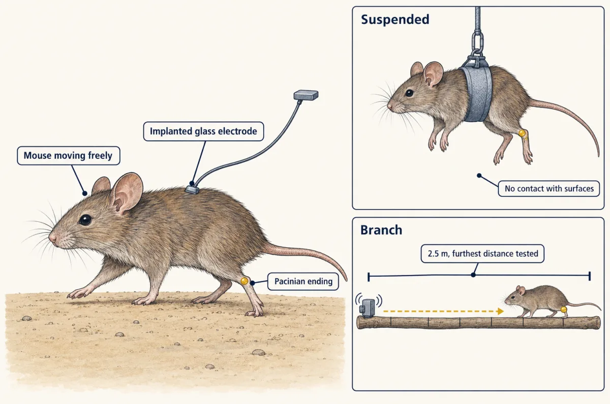
Self-generated input is not erased at the receptors; in this mouse they report it vividly. Any additional cancellation would have to be central, and this study did not measure it.

Design problem

Pacinian afferents in freely moving mice fire during the animal’s own movements. Design the experiments that would tell you whether the central representation of that self-generated vibration is attenuated, and say what each design cannot show.

One way to do it

First, record the same identified afferent class and a downstream station, in the same animal, during self-generated vibration and during externally applied vibration matched in amplitude and frequency content. Attenuation would appear as a smaller downstream response to the self-generated vibration for the same afferent drive. This cannot show how the attenuation arises, and it cannot rule out that the two stimuli differ in some way the matching missed.

Second, replay the recorded self-generated stimulus passively and compare it with the active movement that produced it. A difference points to the motor command or movement-related feedback rather than the stimulus, but not to which.

Third, impose a mismatch between the movement and its sensory consequence, as the vestibular work did, for example by adding an unexpected vibration during the movement, and ask whether attenuation disappears. If it does, the cancellation is conditional on a match. This supports a prediction mechanism in the tested circuit and condition, but a mismatch could also change attention or arousal, so a control for state is needed. None of the designs says whether the human tickle result uses the same mechanism.

Behavioural state, and looming as a test of output pathways

Niell and Stryker (Neuron, 2010) recorded from awake, head-fixed female mice, two to four months old, running or standing on a treadmill. In primary visual cortex most neurons more than doubled their visually evoked firing during running, with stimulus selectivity unchanged. The geniculate input did not show a locomotion-related increase in response magnitude, and some narrow-spiking cells were active during running yet suppressed by visual stimulation. Stringer and colleagues (Science, 2019) imaged on average about 11,000 excitatory neurons per session in awake head-fixed mice and found a high-dimensional ongoing signal partly related to behaviour, with visual stimuli adding representations in dimensions orthogonal to it. Reduced-rank regression, a method that predicts population activity from a small number of behavioural dimensions, found, in separate brain-wide electrode recordings, that predictions from video of the face saturated near 16 dimensions and explained an average of 21.9% of the total variance across areas. That is a relation between movement and activity. Video alone cannot separate a copy of the motor command, reafference from the movement and a correlated change of state, so none of these results is yet an efference-copy pathway. For the visual pathway see visual cortex.

Yilmaz and Meister (Current Biology, 2013) showed freely moving mice, 8 to 12 weeks old, an overhead dark disk whose angular diameter grew from 2 to 20 degrees in 250 ms. The mice escaped or froze, and in the initial flight assay three of ten began escaping within 250 ms, a subset and not an average. The circuit came later. Shang and colleagues (Science, 2015) identified parvalbumin-positive excitatory projection neurons in the mouse superior colliculus as a looming-related defensive pathway, and activating the projection to the parabigeminal nucleus triggered defensive responses. Here parvalbumin marks an excitatory projection neuron, not an interneuron.

In 2018 Shang and colleagues separated two largely distinct projections of those neurons in adult male mice: to the parabigeminal nucleus, where activation produced escape followed by freezing, and to the lateral posterior thalamic nucleus, where activation produced immediate freezing. Bilaterally silencing either target shifted the pattern toward the one tied to the other. In the initial cohort, 44 of 58 mice showed escape followed by freezing. The colliculus is a system with competing outputs, not one fear switch, and these are laboratory behaviours of mice, not a measure of fear in people. For the retinal inputs see retinal cell types and direction selectivity; for restoring lost senses, sensory prostheses.