From Glomeruli to Piriform Cortex

Two mitral cells that take their input from the same glomerulus can fire at the same average rate and still disagree about when in the breathing cycle they fire. If that is true, a glomerulus is a shared address and not a shared message.

Smell and taste ended with receptor neurons converging on glomeruli and the bulb projecting to piriform cortex. This lesson starts at the glomerulus and goes forward, nearly all of it in mice. The question at each stage is what the circuit keeps of the receptor map, what it adds, and what it gives up. How the receptor choice and the axon wiring arise is in olfactory receptor choice, partners, layers and self-avoidance and topographic maps.

Sisters that share an input, and inhibition in the bulb

Mitral and tufted cells are the principal output neurons of the mouse main olfactory bulb. Each sends a primary dendrite into one glomerulus. Cells that send theirs into the same glomerulus are sister cells. Around and beneath them sit interneurons: periglomerular cells, GABAergic cells that work in the glomerular layer, and granule cells, which lack axons and contact the lateral dendrites of mitral and tufted cells.

The key contact is a reciprocal dendrodendritic synapse, one dendrite signalling to another and back. A mitral or tufted dendrite releases glutamate onto the interneuron, and the interneuron releases GABA onto the same dendrite. A reviewer of the rodent literature (Burton, 2017) summarized the consequences: the loop can inhibit the cell that excited it (recurrent inhibition), and because one interneuron touches many output cells, it can inhibit neighbours that share it (lateral inhibition). The principle is the lateral inhibition of sensory coding, built from dendrites. The same review concluded that granule cells alone do not account for all odour-evoked inhibition of mitral and tufted cells, so do not treat granule cells as the whole story.

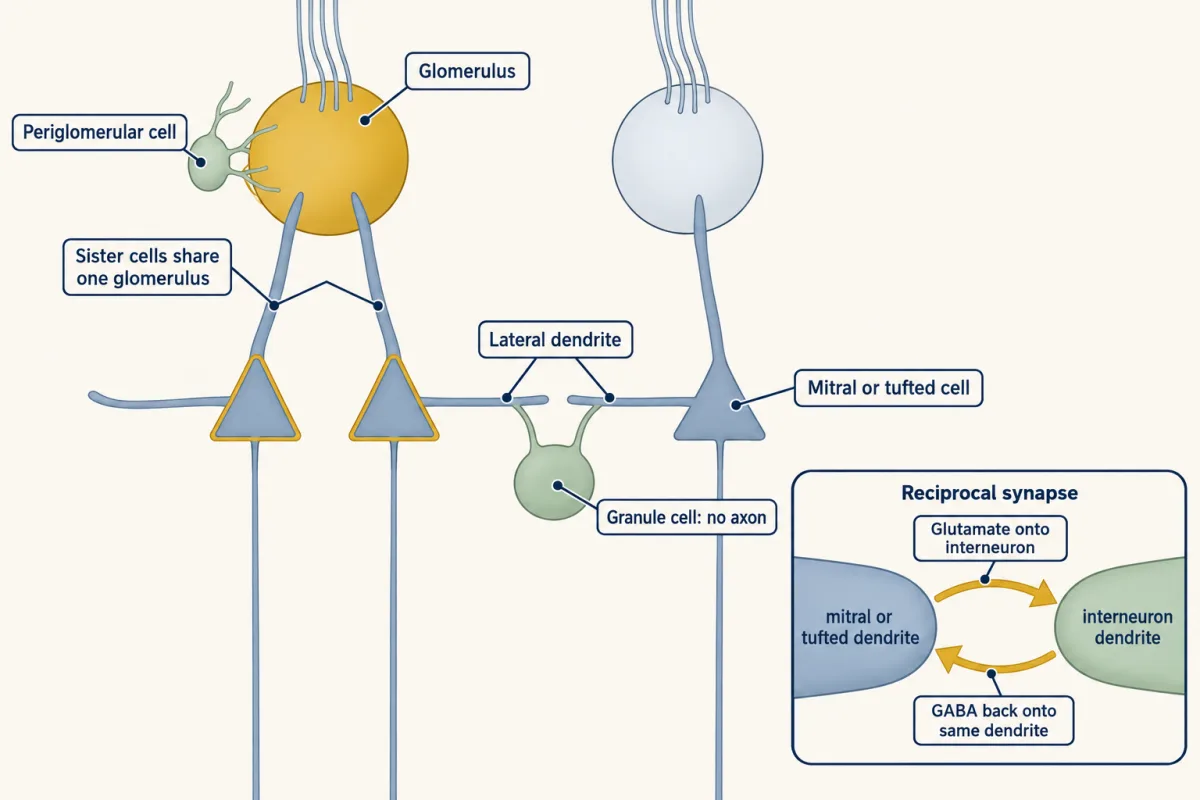
Does a shared glomerulus give sisters a shared code? Dhawale and colleagues (2010) tested this in adult mice, 60 to 400 days old, anaesthetized with ketamine and xylazine. They used a light-based method to find which recorded mitral and tufted cells received input from one parent glomerulus, so sisters were defined by their input and not by how they responded to odours. They then recorded the cells during odour presentation.

Two summaries of the same spikes gave two answers. Counting mean spikes, sister responses were correlated. Looking at spike timing relative to the respiration cycle, odours changed the timing of sisters differently. Rate made them look alike, and timing did not. Both statements belong to the result, and neither is a retreat from the other.

Two cautions. Timing differences do not tell you which synapses produced them, so the experiment does not show that granule-cell inhibition did. And the preparation is anaesthetized, so the same measurement in an awake, sniffing mouse is a separate question.

A cortex with no map, and what it still represents

Mitral and tufted axons reach piriform cortex without a thalamic relay. Stettler and Axel (2009) imaged odour responses in mouse piriform cortex in vivo and found that an odour activated a dispersed ensemble, neurons scattered across the area and not gathered in a patch, and that individual neurons had discontinuous receptive fields. Their result is not a statement that piriform carries no chemical information. It says that the arrangement is not a map of the kind seen in topographic maps.

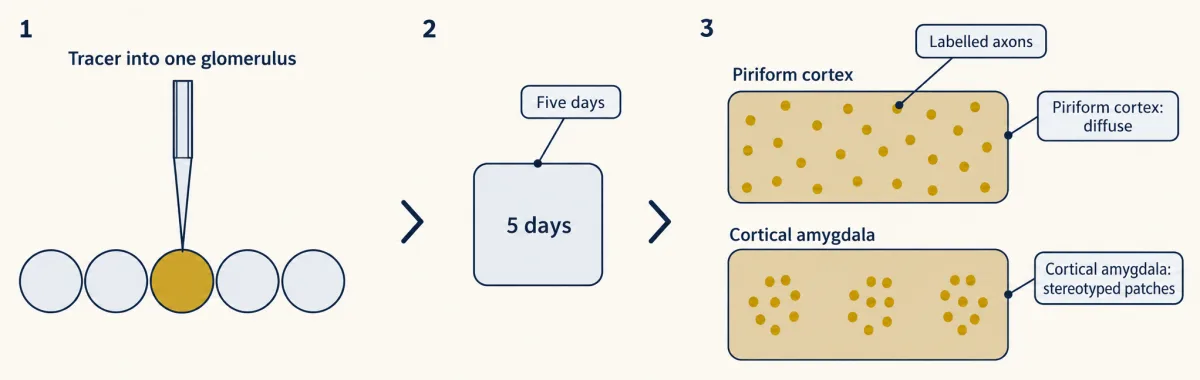
Sosulski and colleagues (2011) asked whether the dispersal begins in the wiring. They electroporated a dextran tracer into a single glomerulus of an adult mouse, waited five days, and imaged the labelled output axons in fixed, flattened cortex and in excised amygdala. In piriform cortex the axons projected diffusely with no apparent spatial preference. In the cortical amygdala the same experiment gave spatially stereotyped patches. So “the bulb projects at random” is wrong in the way that matters: dispersal belongs to one target. Diffuse axons also leave open how individual synapses are chosen, because a tracer image is not a connectivity matrix.

If the anatomy is diffuse, is chemistry lost? Pashkovski and colleagues (2020) imaged piriform layer 2/3 neurons and bulb axon boutons, the terminals of mitral and tufted cells, in male mice 8 to 16 weeks old. The mice were semi-paralysed and ventilated, in a state the authors called wakefulness on EEG criteria, with an imposed 8 Hz sniff cycle, and cortical neurons were tested with three panels of 22 odours (the bulb-bouton comparison used the tiled panel). Both bulb inputs and piriform populations had correlated activity that tracked chemical relationships between odours. The piriform populations clustered related odours more strongly than the bulb inputs did. When the authors attenuated transmission through the cortex’s own associational connections with a genetically targeted silencing tool, the cortical relationships became more like the bulb’s. Passive odour experience could also reshape them.

This is a different kind of map. A spatial map says that similar odours are active in nearby places. A representational geometry says that similar odours evoke similar population patterns wherever the cells sit. The 2020 imaging did not freely sample odours, and fluorescence is not a full record of spikes.

Ensembles that mean something because they were paired

If an odour is an ensemble, what happens if you create one without an odour? Choi and colleagues (2011) expressed channelrhodopsin in subsets of layer 2/3 piriform neurons in awake mice and activated them with light. Pairing the activation with a reward produced one learned behaviour, and pairing it with a shock produced the opposite. Ensembles of as few as 300 neurons could drive a learned response, weakly (flight in about 30 percent of aversive-task trials at about 300 cells and about 95 percent above 500), and mice could learn to discriminate different activated subpopulations. (For optogenetic tools, see hacking the cell; for learned associations, synaptic plasticity and memory consolidation.)

What this shows is that arbitrary piriform activity can acquire learned behavioural meaning, which is sufficiency for an association. It does not show that the mice smelled something, and the authors withheld the claim that their artificial network reproduced natural odour processing. The figure of 300 is the smallest effective ensemble tested here, with a weaker response than larger ensembles, and not the size of a natural odour representation.

Worked problem, part a: the stimulus. The aversive-conditioning photostimulus used 20 Hz pulses of 25 ms each. Suppose, as an exercise, a train lasts 3 s with one pulse starting each period. The 3 s is our assumption.

Step 1: period. 1/20 s = 50 ms. Step 2: pulses. 20 s⁻¹ x 3 s = 60 pulses. Step 3: off-time per period. 50 ms - 25 ms = 25 ms. Step 4: duty cycle. 25/50 = 0.50. Step 5: light-on time. 60 x 25 ms = 1,500 ms = 1.5 s. Check: 3 s x 0.50 = 1.5 s.

These are stimulus quantities. They do not say that neurons fired 60 spikes.

Pulse frequency 20 Hz Pulse width 25 ms Train duration 3 s (our assumption)

Period = 1/f

Pulses = f × duration

Off-time per period

Duty cycle = on ÷ period

Total light-on time

Check: duration × duty

In this sketch: square light pulses, one pulse starting each period, stimulus quantities only, no neural response modelled. The drawing is computed from the three settings and is not a recording.

Rule to keep: duty cycle = pulse width ÷ period, and light-on time = pulses × width = duration × duty. These are stimulus quantities, not spike counts.

Representations that drift

If an odour has an ensemble, you might expect it to stay the same. Schoonover and colleagues (2021) recorded single units in mouse piriform cortex over days to weeks. Odour-evoked responses drifted. A classifier trained on the first recording day approached chance performance by 32 days. Daily exposure to an odour slowed the drift, and fear conditioning did not stabilize the responses. The 32 days is the point where this classifier approached chance, not a time constant.

Drift does not mean that an animal’s smell changed. A decoder is a tool the experimenter holds, and a downstream circuit may read a moving population consistently. The finding does change what a cortical ensemble can mean, because the fixed address of the textbook ensemble is not what these recordings show.

Design problem

A classifier trained on day 1 piriform responses decodes odours well on day 1 and near chance a month later. Design the experiments that distinguish a changing neural code from a changing recording, and say what the result does not show.

One way to do it

Is the recording stable? Check that the same units are tracked: compare waveform shape, isolation quality and baseline firing across days, and repeat with a subset that is clearly the same cells.

Is the failure about the decoder? Train a new decoder on each day and compare it with the frozen day-1 decoder. If daily decoders work and the frozen one fails, odour information is present every day while the mapping changed. If daily decoders also fail late, the recording itself has probably lost information.

Does behaviour drift too? Test the animal’s discrimination of the same odours on the same days. If behaviour holds steady while the decoder fails, a downstream reader is coping with the change.

What controls drift? Compare animals with daily exposure, with fear conditioning and with neither, as the paper did, and ask which factor changes the rate.

What stays unproven. A failed decoder alone does not show a changed percept, and a change in code does not show which synapses changed.

Learned maps, and smell loss in people

A different route to odour structure skips the brain. Lee, Mayhew and colleagues (2023) trained a graph neural network on approximately 5,000 labelled molecules and represented every molecule as a point in 256 learned dimensions, a principal odor map. This is a computational embedding, not anatomy.

Worked problem, part b: the prospective test. A human panel characterized 400 new odorants, and 323 were retained for the final evaluation with no retraining.

Step 1: fraction retained. 323/400 = 0.8075, or 80.75 percent. Step 2: what 53 percent counts. For 53 percent of evaluated molecules, the model’s profile was closer to the panel mean than the median panellist’s was. Step 3: how many molecules. 0.53 x 323 = about 171. It is not classification accuracy.

The map did not predict suprathreshold intensity as concentration varied, and the roughly 500,000-molecule picture plots predictions.

In people, smell loss has been studied from the epithelium to the clinic. Early in the pandemic Brann and colleagues (2020) found the ACE2 entry gene in non-neuronal olfactory cells and localized ACE2 protein to sustentacular cells in mouse dorsal epithelium, not in sensory neurons, which suggested non-neuronal mechanisms. Khan and colleagues (2021) examined adult postmortem tissue from people who had died with COVID-19 and found sustentacular cells to be the main olfactory mucosal target, with no evidence of infection of sensory neurons or the bulb parenchyma in their samples. They allowed that mechanisms may differ between people. Do not say the virus infects olfactory neurons and travels into the brain.

Smell test scores also predict disease in cohorts. In the Health ABC study of 2,462 community-dwelling people aged 70 to 79 at enrolment, the lowest tertile of a smell identification test had a Parkinson disease hazard ratio of 4.8 against the highest tertile (95% CI 2.0 to 11.2, from only 42 incident cases; Chen and colleagues, 2017). In a North Manhattan cohort, lower smell scores were associated with later Alzheimer dementia (Devanand and colleagues, 2015). These are associations, not diagnoses, and smell loss has other causes such as chronic rhinosinusitis.

Ahead: taste coding takes the same question to a sense with few receptors, and multisensory integration and prediction asks how smell combines with other senses.